raised cosine basis functions

This was a post I wrote for members of my lab, as we were trying to find out why a particular set of functions was chosen. The particulars aren't important, but I thought the interface was nice. Play around a bit. The changes are really simple, but solve what is oddly my biggest frustration in reading papers: jumping from figure refs to figures themselves and back again, with repetitive captions. We optimized papers for print (and did a great job), but we really haven't changed now that we have this new medium. This was hacked together with some jquery and jekyll and mathjax; someone who codes js for a living might do better with knockout or tangle. Incidentally, if scientific journals helped me do more than I can accomplish in LaTeX, I'd be more sympathetic to their dominance. So: click on things that look clickable, tell me what you think. It sounds really simple, but the ability to view a figure without losing context helps me immeasurably.

Papers

I read through the methods in three papers because I was bothered by my hand-wavy justification:

Nature retina paper

Nature retina supp

JNeuroscience retina paper

Neuron modeling paper

The number one thing we’re probably interested in for spike-history basis functions is a basis which describes the spike-triggered psth with as few basis functions as possible. Time dilation and using a raised cosine have certain advantages in this regard, and we’ll discuss them below.

Understanding Time Dilation

The Neuron paper does not use raised cosine basis functions, but a very similar kind and they explain the reason for using a stretched basis function best. They note that they tried using a fourier basis to represent an empirically observed filter. A fourier basis would in principle give you varying degrees of temporal precision, with phase-shifted cosines of different frequencies, able to approximate an arbitrary function with arbitrary precision as we all know. However, they found that they needed many more basis functions to approximate empirically observed filters than with stretched versions. Their explanation was that firing rate was more highly variable close to the trigger event than further away from it, due to variability in stimulus, neural activity, or some other source. So they induced stretching, and wanted to be “principled”:

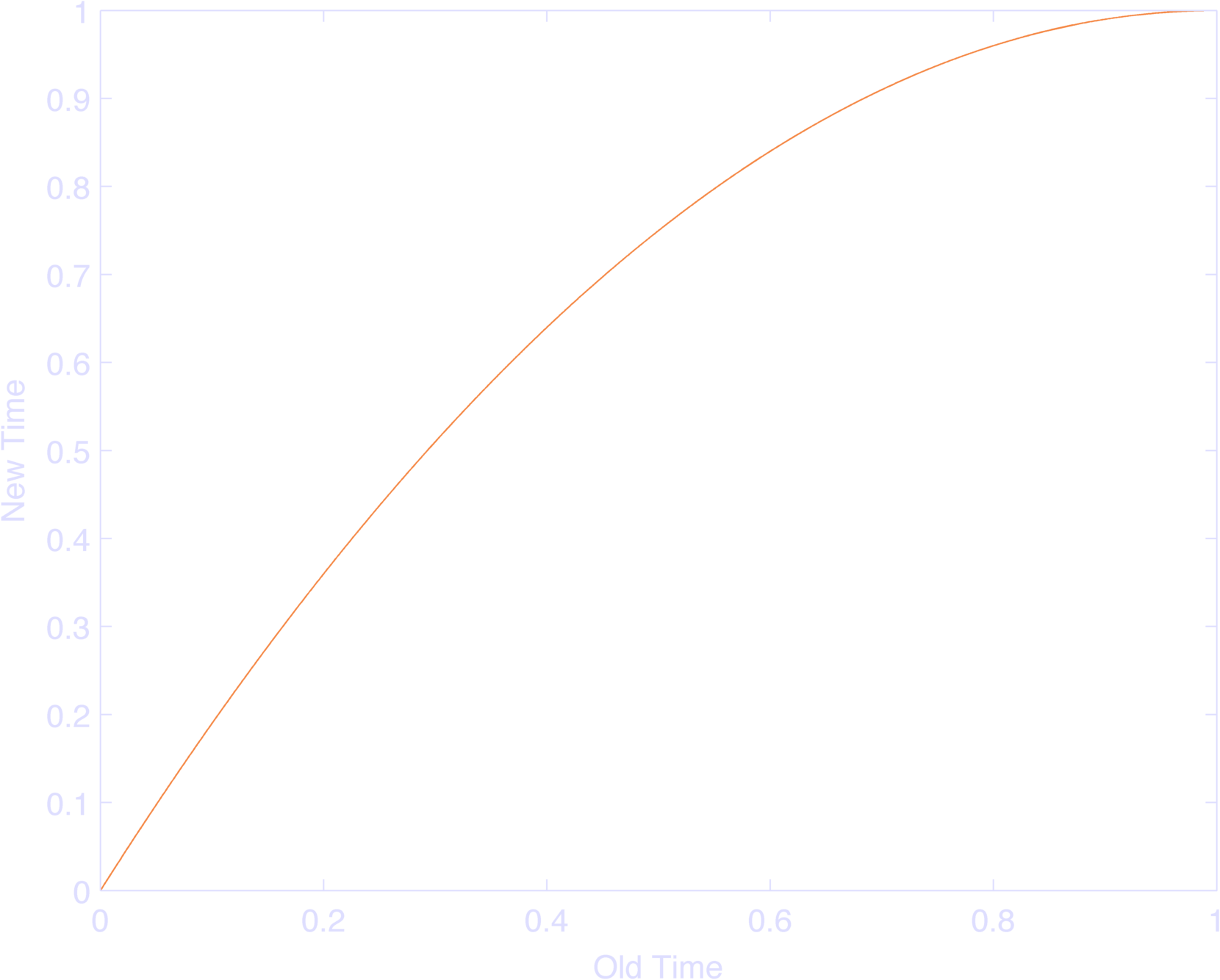
A normal fourier basis would have, say, $\sin( \pi f_k t ) $ for the kth basis function. They basically replaced $t$ with $2 t - t^2$, with $t$ ranging from $0$ to $1$ which makes the entire input range from 0 to 1 (Figure 1), but more and more slowly as you get closer to $1$, from a rate of $1$ to a rate of $0$. This makes the basis function as a whole oscillate at $\pi f_k$ rad/s at $t=0$, and $0$ rad/s at $t=1$. Moreover, the rate of frequency change is linear in time. NIFTY TRICK!

The point is that they showed empirically that their stretched model did better than a regular fourier basis which makes sense in retrospect, but is better than the hand-waving I was doing.

Raised Cosines

The Pillow 2005 JNeuroscience paper did a similar thing, but induced a nonlinearity via a log function instead of a polynomial, and used cosine functions instead of sine functions.

Decomposing what’s going on, we have:

$$\frac{1}{2} ( \cos( \log( t + \psi ) - \varphi_i ) + 1)$$

So if I have a cosine and I add 1 I get a function going from 0 to 2. So divide that by two and I get a function going from 0 to 1. So I’ll concern myself with:

$$ \cos( \log( t + \psi ) - \varphi_i ) $$

Looking at $\log( t + \psi ) $, where $ t $ goes from 0 to $ \tau $, I note that this dilates time: Near 0, the log has near infinite slope, as t increases, the slope decreases. This we all know. $\psi $ will shift this function left with positive values of $ \psi $. The main point of $ \psi $ is to change the range of log for given values of $t$, and the rate at which those values change. If you don’t like your function starting at -infinity, shift it to the left a bit; if you want it very linear, shift it to the left a lot. So whereas the Keat paper scaled frequencies with a factor of 1 to 0, this function scales frequencies with a range of infinity at log(0) to ~1 at log(1) to 1/2 at log(2) to 1/10 at log(10) (yay, derivatives). More plainly, it’s SUPERFAST to MEH ability to fit the model to changes as you get farther from the trigger. Changing $ \psi $ would change your model, because you’re necessarily changing the timescale of your basis functions.

But why raised cosines?

It might be helpful to compare the cosine choice to the choice in the Keat paper Pillow references. In the Keat paper, they let each basis function varies over the entire time-scale, so that you are still doing ‘fourier analysis’, but it’s as if you get a basis with a slightly decreased frequency set from one time-point to the next. In the Pillow paper, they set the basis functions to 0 except wherever $ \log( t + \psi ) $ ranges from $ \varphi - \pi $ to $ \varphi + \pi $. This way they get one cosine cycle, or a single raised bump. This is nice, so that they get a single time-lag that each bump is focused on, and a single time-scale, with time-scale depending on time-lag. You also get a single bump with a peak at 0 phase which makes the peak easy to control. There isn’t a good sense of ‘peak’ in the Keat paper, since each basis function continues to oscillate.

Raised cosines also allow for the choice of peaks in the JNeuroscience “so that the basis vectors ‘tile,’ or sum to 1, allowing for phase-invariant (on a log-time axis) representation” of the spike-history term. Looking first at the “sum to 1” part, we note that if you sum two cosines that are exactly out of phase they sum to 0 (e.g. $\cos( x ) + \cos( x + \pi ) $ ). Two raised cosines will sum to a constant. In the log-time axis, since we need to ensure that each cosine bump dilates at the same rate, so that the sum at any given point will still be a constant. The easiest way to do this is to (a) make sure that each raised cosine has access to the same time scale and (b) make sure that each raised cosine’s phase is offset by $\pi$. If we have more than two cosine bumps, we need to make sure that each cosine bump only overlaps one other bump at a time (we’ll relax this constraint later). So if you care about basis functions “tiling” the input space, raised cosine basis functions make this easy.

So how do we get them to work?

It’s also helpful to see how useful they are by how they work.

With two basis functions, to get them to sum to one, I’d write:

$$ \frac{1}{2} \cos( x + \pi ) + \frac{1}{2} \cos( x ) + 1 = 1 $$

To specify the basis functions with arbitrary zeros, I’d write:

$$ \frac{1}{2} \cos( (x - c_1) + \frac{1}{2} \cos( x - c_2 ) + 1 = 1 $$

while requiring that $ c_1 $ and $c_2$ are $\pi$ apart.

The problem with this approach is that it doesn’t let us have more than two bases, since adding a third cosine will break the requirement that the bases sum to 1. But if we restrict each cosine to only be active between $\pm \pi $ then we get nice overlapping, and we can use as many cosines (now cosine bumps) as we wish, because at any given point in time, only two cosines will overlap.

Now we just need to make sure that we keep only one cycle of the cosine function centered at phase 0. In matlab, here’s what I would do (different than Konrad’s code):

t = linspace(0,1,1000);
nBas = 5;

cSt = 0;
cEnd = 1;
db = (cEnd - cSt) /
     (nBases-1)
c = cSt:db:cEnd;
 
bas = nan(length(phi),length(t));
for k = 1:length(phi)
  bas(k,:) = ( cos( ...
    max(-pi, 
    min(pi,pi*(t - c(k))/(db) )...
    ) ) + 1) / 2;
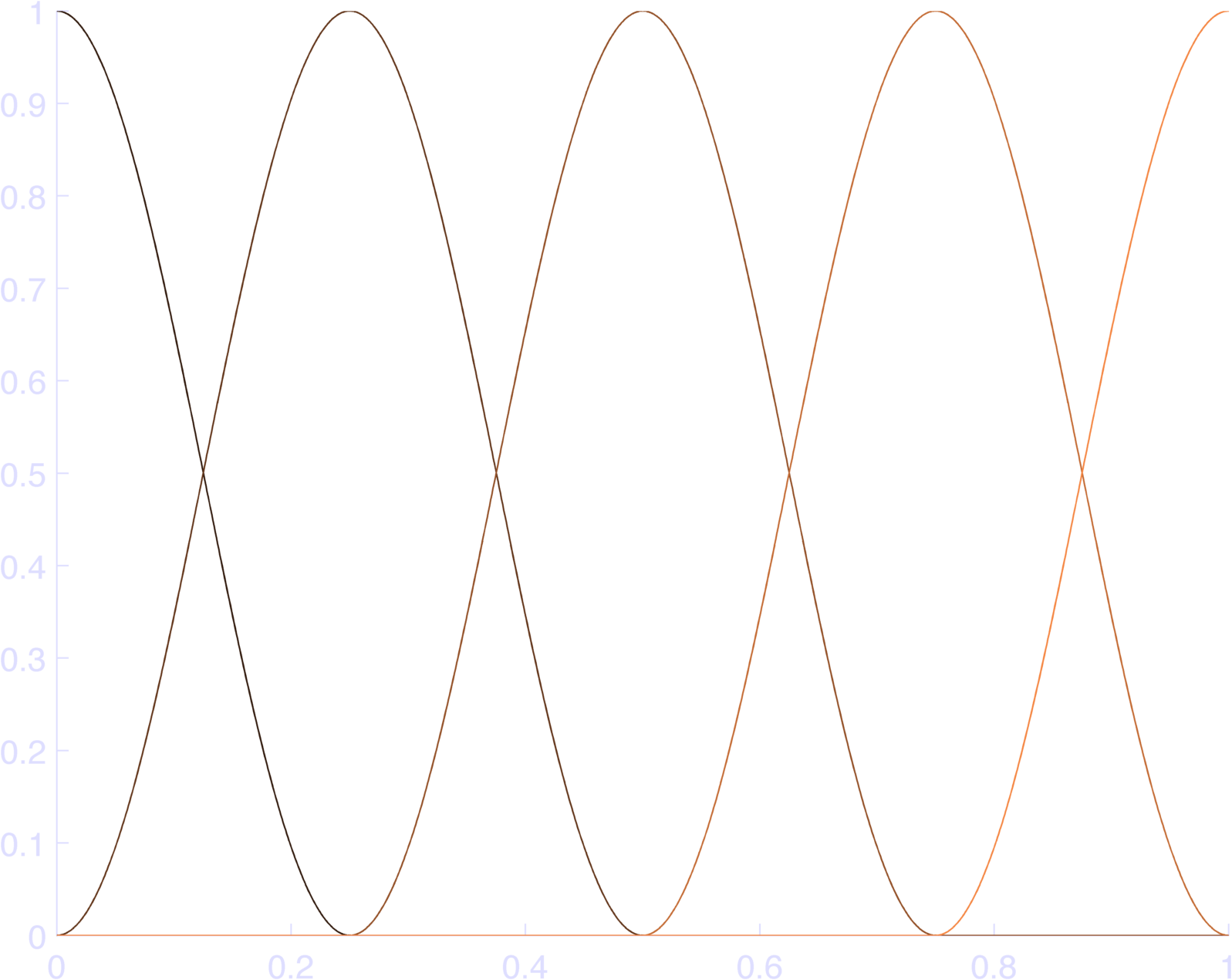
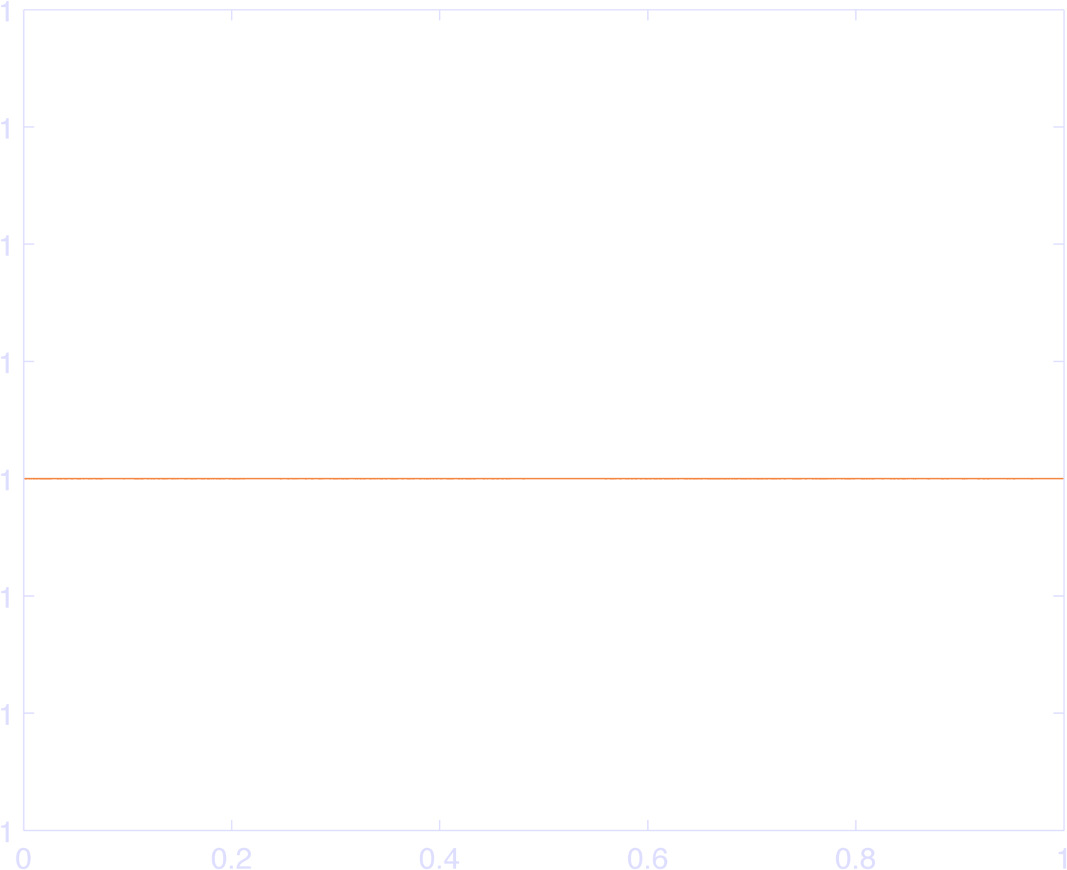
end

You can see the results in Figure 2, which sum to 1 (Figure 3).

This is great, but what about the log-time?

To reintroduce the log, we do two things. First, let $ c_i $ be the center in the log-time axis where we want the peak of the $i$th cosine bump, at regular intervals. If these interval are all $d$ apart, then we want the log-transformed time to go in for $x$ in the above equation. The best way to do this might be:

$$ x = \frac{\log( t + b ) - c_i}{d}\pi $$

This ensures that once you get to the next center in log-time, you will be at exactly $\pi$, and when you get to the previous one, you will be at exactly $-\pi$. This fulfills the requirement (a) above, that each cosine has access to the same time scale since $\log( t + b )$ does not depend on the basis function, and (b) that the offset is still constrained to be $\pi$, even though in time we could have chosen basis distance we wished.

The weird max-min code idiom ensures that each raised cosine bump is 0 outside of $\pm \pi$, since the input to $\cos$ is set to $\pm \pi$ outside this range, and $\cos( \pm \pi )$ is 0 at these values. Thus, they “tile” the inputs. YAY. Go ahead and plot the sum of the bas, it’s identically 1.

So here’s my implementation:

b = 0.1;
t = linspace(0,1,1000);
nlin  = inline('log(x+eps)');
nt = nlin(t + b);
nBases = 5;
cSt = nt(1);
cEnd = nt(end);
db = (cEnd - cSt) / (nBases-1)
c = cSt:db:cEnd;

bas = nan(nBases,length(t));
for k = 1:nBases
  bas(k,:) = ( cos( ...
    max(-pi, min(pi,(nt - c(k))*pi/(db) )) ) ...
    + 1) / 2;
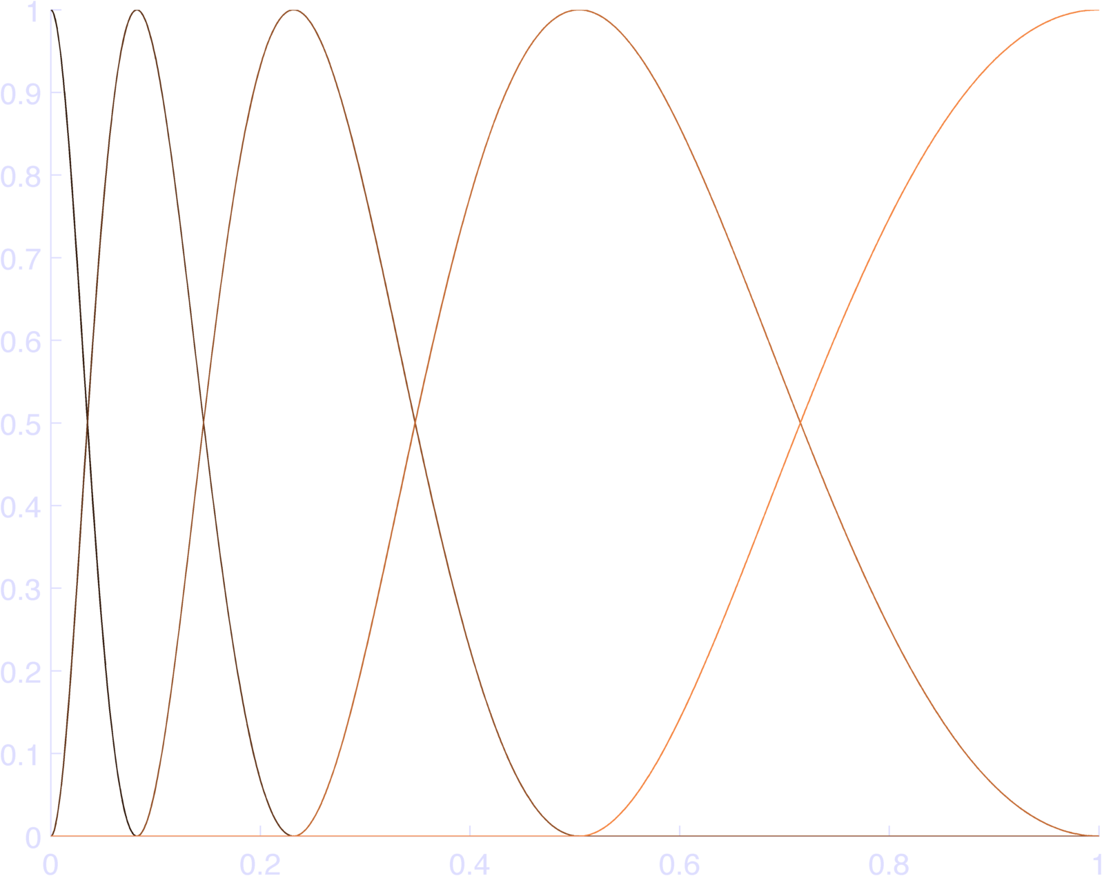
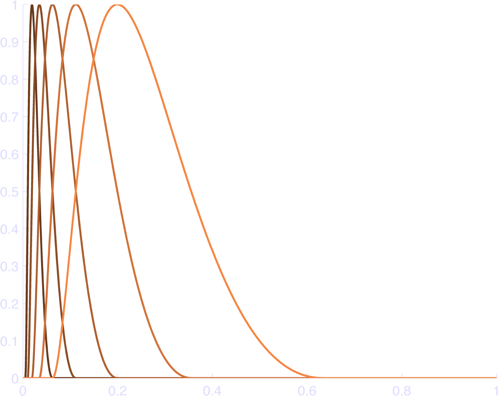
end

This makes pretty bases, as in Figure 4. You can check that this sums to 1 at each individual time point in Figure 5.

Additional Modifications

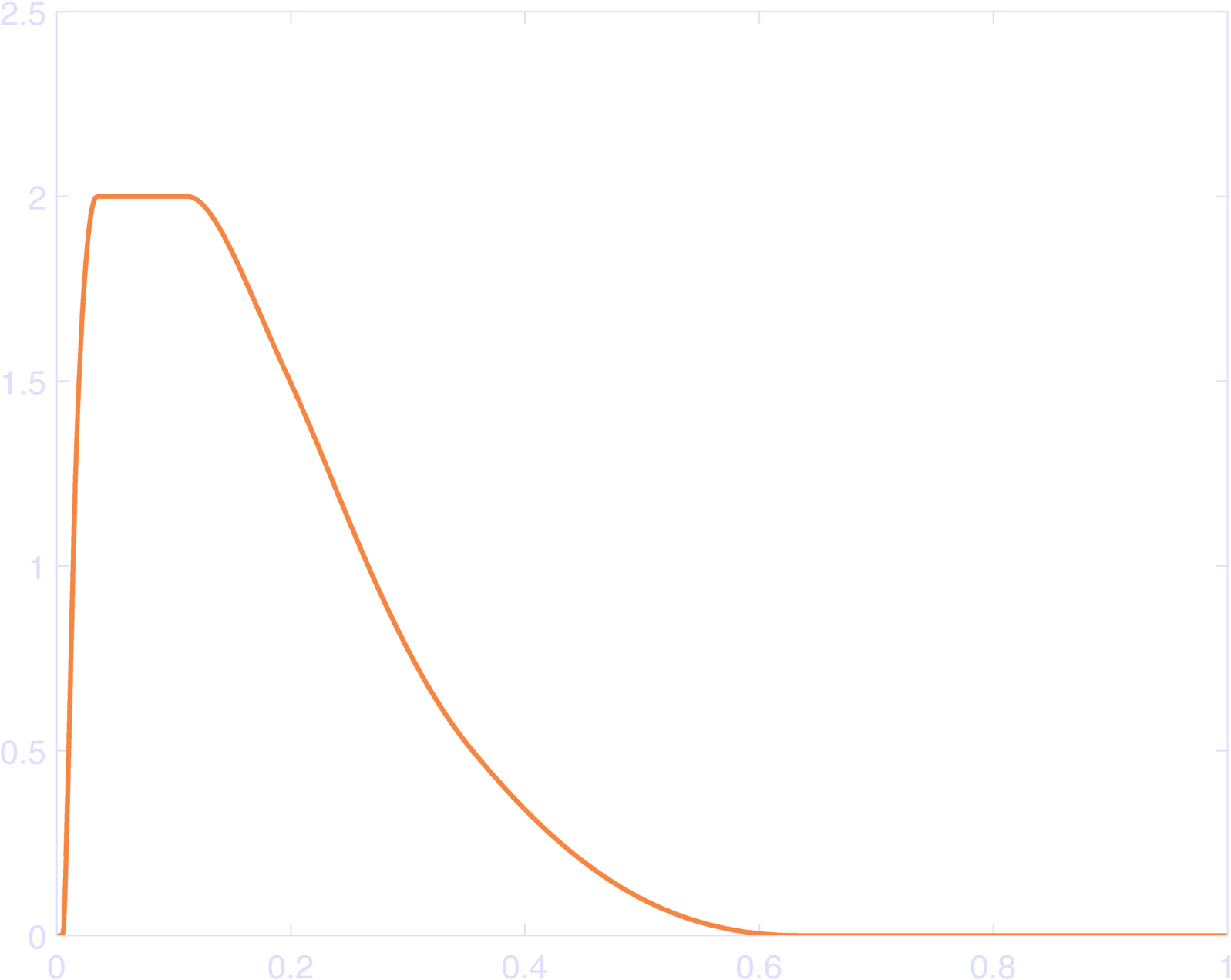
There are two slight issues with this approach. First we might not like to have a basis-center at the last point in time. To avoid this, we can relax the constraint that our bases must sum to 1 at each point in time, so that we can set the first and/or last basis-centers to be not quite the last point in the log-time axis. Figure 6 gives an example of this. It does have the property that it sums to a constant over a smaller range (Figure 7).

The second issue is that we might want more overlapping between bases, so that we can vary them more independently. For instance, if a function had a peak at 0.15 in Figure 4, we might have to scale the cosine bumps on either side twice as much as if there happened to be a bump right at 0.15, which has an affect on a wide area of time. To get around this, we can change the cosine bumps so that they range from $-\pi$ to $\pi$ as the log-transformed time runs from two basis centers on the left to two basis centers on the right. The point is that we must choose it so that at any given point we have an even number of cosines, with alternating signs, so that they sum to a constant. There might be other methods which also create a cancellation effect, but so I might be missing something. Alternatively, we could just increase the number of basis functions, but this has a slightly different effect. Figure 6 shows the affect of doubling the overlap.

Finally, we can, as was done in the Pillow et al 2008 Nature paper, set the location of the peaks to specific phases, and remove them from the scaling and transfer them to radians directly. So instead of inputing to the cosine